It contains high-level data structures and manipulation tools designed to make data analysis fast and easy in Python. pandas is built on top of NumP and makes it easy to use in NumPy-centric applications.
Data structures with labeled axes supporting automatic or explicit data alignment. This prevents common errors resulting from misaligned data and working with differently-indexed data coming from different sources.
Integrated time series functionality.
The same data structures handle both time series data and non-time series data.
Arithmetic operations and reductions (like summing across an axis) would pass on the metadata (axis labels).
Flexible handling of missing data.
Merge and other relational operations found in popular database databases (SQLbased, for example).
number = [ 1 , 2 , 3 ]
pd . Series ( number )
animals = [ 'Tiger' , 'Bear' , None ]
pd . Series ( animals )
0    Tiger
1     Bear
2     None
dtype: object
import numpy as np
np . nan == None
sports = { 'Archery' : 'Bhutan' ,
'Golf' : 'Scotland' ,
'Sumo' : 'Japan' ,
'Taekwondo' : 'South Korea' }
s = pd . Series ( sports )
s
Archery           Bhutan
Golf            Scotland
Sumo               Japan
Taekwondo    South Korea
dtype: object
Index(['Archery', 'Golf', 'Sumo', 'Taekwondo'], dtype='object')
s = pd . Series ([ 'Tiger' , 'Bear' , 'Moose' ], index = [ 'India' , 'America' , 'Canada' ])
s
India      Tiger
America     Bear
Canada     Moose
dtype: object
sports = { 'Archery' : 'Bhutan' ,
'Golf' : 'Scotland' ,
'Sumo' : 'Japan' ,
'Taekwondo' : 'South Korea' }
s = pd . Series ( sports , index = [ 'Golf' , 'Sumo' , 'Hockey' ])
s
Golf      Scotland
Sumo         Japan
Hockey         NaN
dtype: object
sports = { 'Archery' : 'Bhutan' ,
'Golf' : 'Scotland' ,
'Sumo' : 'Japan' ,
'Taekwondo' : 'South Korea' }
s = pd . Series ( sports )
s
Archery           Bhutan
Golf            Scotland
Sumo               Japan
Taekwondo    South Korea
dtype: object
sports = { 99 : 'Bhutan' ,
100 : 'Scotland' ,
101 : 'Japan' ,
102 : 'South Korea' }
s = pd . Series ( sports )
s [ 0 ] #This won't call s.iloc[0] as one might expect, it generates an error instead
---------------------------------------------------------------------------

KeyError                                  Traceback (most recent call last)

c:\Users\LENOVO\AppData\Local\Programs\Python\Python39\lib\site-packages\pandas\core\indexes\base.py in get_loc(self, key, method, tolerance)
   3360             try:
-> 3361                 return self._engine.get_loc(casted_key)
   3362             except KeyError as err:


c:\Users\LENOVO\AppData\Local\Programs\Python\Python39\lib\site-packages\pandas\_libs\index.pyx in pandas._libs.index.IndexEngine.get_loc()


c:\Users\LENOVO\AppData\Local\Programs\Python\Python39\lib\site-packages\pandas\_libs\index.pyx in pandas._libs.index.IndexEngine.get_loc()


pandas\_libs\hashtable_class_helper.pxi in pandas._libs.hashtable.Int64HashTable.get_item()


pandas\_libs\hashtable_class_helper.pxi in pandas._libs.hashtable.Int64HashTable.get_item()


KeyError: 0


The above exception was the direct cause of the following exception:


KeyError                                  Traceback (most recent call last)

~\AppData\Local\Temp/ipykernel_7512/4087325533.py in <module>
----> 1 s[0] #This won't call s.iloc[0] as one might expect, it generates an error instead


c:\Users\LENOVO\AppData\Local\Programs\Python\Python39\lib\site-packages\pandas\core\series.py in __getitem__(self, key)
    940
    941         elif key_is_scalar:
--> 942             return self._get_value(key)
    943
    944         if is_hashable(key):


c:\Users\LENOVO\AppData\Local\Programs\Python\Python39\lib\site-packages\pandas\core\series.py in _get_value(self, label, takeable)
   1049
   1050         # Similar to Index.get_value, but we do not fall back to positional
-> 1051         loc = self.index.get_loc(label)
   1052         return self.index._get_values_for_loc(self, loc, label)
   1053


c:\Users\LENOVO\AppData\Local\Programs\Python\Python39\lib\site-packages\pandas\core\indexes\base.py in get_loc(self, key, method, tolerance)
   3361                 return self._engine.get_loc(casted_key)
   3362             except KeyError as err:
-> 3363                 raise KeyError(key) from err
   3364
   3365         if is_scalar(key) and isna(key) and not self.hasnans:


KeyError: 0
s = pd . Series ([ 100.00 , 120.00 , 101.00 , 3.00 ])
np . sum ( s )
0    100.0
1    120.0
2    101.0
dtype: float64
s = pd . Series ([ 1 , 2 , 3 ])
s . loc [ 'Animal' ] = 'Bears'
s
0             1
1             2
2             3
Animal    Bears
dtype: object
original_sports = pd . Series ({ 'Archery' : 'Bhutan' ,
'Golf' : 'Scotland' ,
'Sumo' : 'Japan' ,
'Taekwondo' : 'South Korea' })
cricket_loving_countries = pd . Series ([ 'Australia' ,
'Barbados' ,
'Pakistan' ,
'England' ],
index = [ 'Cricket' ,
'Cricket' ,
'Cricket' ,
'Cricket' ])
all_countries = original_sports . append ( cricket_loving_countries )
Archery           Bhutan
Golf            Scotland
Sumo               Japan
Taekwondo    South Korea
dtype: object
Cricket    Australia
Cricket     Barbados
Cricket     Pakistan
Cricket      England
dtype: object
Archery           Bhutan
Golf            Scotland
Sumo               Japan
Taekwondo    South Korea
Cricket        Australia
Cricket         Barbados
Cricket         Pakistan
Cricket          England
dtype: object
all_countries . loc [ 'Cricket' ]
Cricket    Australia
Cricket     Barbados
Cricket     Pakistan
Cricket      England
dtype: object
purchase_1 = pd . Series ({ 'Name' : 'Chris' ,
'Item Purchased' : 'Dog Food' ,
'Cost' : 22.50 })
purchase_2 = pd . Series ({ 'Name' : 'Kevyn' ,
'Item Purchased' : 'Kitty Litter' ,
'Cost' : 2.50 })
purchase_3 = pd . Series ({ 'Name' : 'Vinod' ,
'Item Purchased' : 'Bird Seed' ,
'Cost' : 5.00 })
df = pd . DataFrame ([ purchase_1 , purchase_2 , purchase_3 ], index = [ 'Store 1' , 'Store 1' , 'Store 2' ])
df . head ()
Name
Item Purchased
Cost
Store 1
Chris
Dog Food
22.5
Store 1
Kevyn
Kitty Litter
2.5
Store 2
Vinod
Bird Seed
5.0
Name                  Vinod
Item Purchased    Bird Seed
Cost                    5.0
Name: Store 2, dtype: object
pandas.core.series.Series
Name
Item Purchased
Cost
Store 1
Chris
Dog Food
22.5
Store 1
Kevyn
Kitty Litter
2.5
df . loc [ 'Store 1' , 'Cost' ]
Store 1    22.5
Store 1     2.5
Name: Cost, dtype: float64
Store 1
Store 1
Store 2
Name
Chris
Kevyn
Vinod
Item Purchased
Dog Food
Kitty Litter
Bird Seed
Cost
22.5
2.5
5.0
Store 1    22.5
Store 1     2.5
Store 2     5.0
Name: Cost, dtype: object
Store 1    22.5
Store 1     2.5
Store 2     5.0
Name: Cost, dtype: float64
df . loc [ 'Store 1' ][ 'Cost' ]
Store 1    22.5
Store 1     2.5
Name: Cost, dtype: float64
df . loc [:,[ 'Name' , 'Cost' ]]
Name
Cost
Store 1
Chris
22.5
Store 1
Kevyn
2.5
Store 2
Vinod
5.0
Name
Item Purchased
Cost
Store 1
Chris
Dog Food
22.5
Store 1
Kevyn
Kitty Litter
2.5
Store 2
Vinod
Bird Seed
5.0
copy_df = df . copy ()
copy_df = copy_df . drop ( 'Store 1' )
#copy_df.drop('Store 1', inplace=True)
copy_df
Name
Item Purchased
Cost
Location
Store 2
Vinod
Bird Seed
5.0
None
del copy_df [ 'Name' ]
copy_df
Item Purchased
Cost
Store 2
Bird Seed
5.0
Name
Item Purchased
Cost
Location
Store 1
Chris
Dog Food
22.5
None
Store 1
Kevyn
Kitty Litter
2.5
None
Store 2
Vinod
Bird Seed
5.0
None
Store 1    22.5
Store 1     2.5
Store 2     5.0
Name: Cost, dtype: float64
Store 1    24.5
Store 1     4.5
Store 2     7.0
Name: Cost, dtype: float64
Name
Item Purchased
Cost
Location
Store 1
Chris
Dog Food
24.5
None
Store 1
Kevyn
Kitty Litter
4.5
None
Store 2
Vinod
Bird Seed
7.0
None
df = pd . read_csv ( 'olympics.csv' , index_col = 0 , skiprows = 1 )
df . head ()
№ Summer
01 !
02 !
03 !
Total
№ Winter
01 !.1
02 !.1
03 !.1
Total.1
№ Games
01 !.2
02 !.2
03 !.2
Combined total
Afghanistan (AFG)
13
0
0
2
2
0
0
0
0
0
13
0
0
2
2
Algeria (ALG)
12
5
2
8
15
3
0
0
0
0
15
5
2
8
15
Argentina (ARG)
23
18
24
28
70
18
0
0
0
0
41
18
24
28
70
Armenia (ARM)
5
1
2
9
12
6
0
0
0
0
11
1
2
9
12
Australasia (ANZ) [ANZ]
2
3
4
5
12
0
0
0
0
0
2
3
4
5
12
Index(['№ Summer', '01 !', '02 !', '03 !', 'Total', '№ Winter', '01 !.1',
       '02 !.1', '03 !.1', 'Total.1', '№ Games', '01 !.2', '02 !.2', '03 !.2',
       'Combined total'],
      dtype='object')
<class 'pandas.core.frame.DataFrame'>
Index: 147 entries, Afghanistan (AFG) to Totals
Data columns (total 15 columns):
 #   Column          Non-Null Count  Dtype
---  ------          --------------  -----
 0   № Summer        147 non-null    int64
 1   01 !            147 non-null    int64
 2   02 !            147 non-null    int64
 3   03 !            147 non-null    int64
 4   Total           147 non-null    int64
 5   № Winter        147 non-null    int64
 6   01 !.1          147 non-null    int64
 7   02 !.1          147 non-null    int64
 8   03 !.1          147 non-null    int64
 9   Total.1         147 non-null    int64
 10  № Games         147 non-null    int64
 11  01 !.2          147 non-null    int64
 12  02 !.2          147 non-null    int64
 13  03 !.2          147 non-null    int64
 14  Combined total  147 non-null    int64
dtypes: int64(15)
memory usage: 18.4+ KB
for col in df . columns :
if col [: 2 ] == '01' :
df . rename ( columns = { col : 'Gold' + col [ 4 :]}, inplace = True )
if col [: 2 ] == '02' :
df . rename ( columns = { col : 'Silver' + col [ 4 :]}, inplace = True )
if col [: 2 ] == '03' :
df . rename ( columns = { col : 'Bronze' + col [ 4 :]}, inplace = True )
if col [: 1 ] == '№' :
df . rename ( columns = { col : '#' + col [ 1 :]}, inplace = True )
df . head ()
# Summer
Gold
Silver
Bronze
Total
# Winter
Gold.1
Silver.1
Bronze.1
Total.1
# Games
Gold.2
Silver.2
Bronze.2
Combined total
Afghanistan (AFG)
13
0
0
2
2
0
0
0
0
0
13
0
0
2
2
Algeria (ALG)
12
5
2
8
15
3
0
0
0
0
15
5
2
8
15
Argentina (ARG)
23
18
24
28
70
18
0
0
0
0
41
18
24
28
70
Armenia (ARM)
5
1
2
9
12
6
0
0
0
0
11
1
2
9
12
Australasia (ANZ) [ANZ]
2
3
4
5
12
0
0
0
0
0
2
3
4
5
12
# Summer
Gold
Silver
Bronze
Total
# Winter
Gold.1
Silver.1
Bronze.1
Total.1
# Games
Gold.2
Silver.2
Bronze.2
Combined total
count
147.000000
147.000000
147.000000
147.000000
147.000000
147.000000
147.000000
147.000000
147.000000
147.000000
147.000000
147.000000
147.000000
147.000000
147.000000
mean
13.476190
65.428571
64.965986
69.795918
200.190476
6.700680
13.047619
13.034014
12.897959
38.979592
20.176871
78.476190
78.000000
82.693878
239.170068
std
7.072359
405.549990
399.309960
427.187344
1231.306297
7.433186
80.799204
80.634421
79.588388
240.917324
13.257048
485.013378
478.860334
505.855110
1469.067883
min
1.000000
0.000000
0.000000
0.000000
0.000000
0.000000
0.000000
0.000000
0.000000
0.000000
1.000000
0.000000
0.000000
0.000000
1.000000
25%
8.000000
0.000000
1.000000
1.000000
2.000000
0.000000
0.000000
0.000000
0.000000
0.000000
11.000000
0.000000
1.000000
1.000000
2.500000
50%
13.000000
3.000000
4.000000
6.000000
12.000000
5.000000
0.000000
0.000000
0.000000
0.000000
15.000000
3.000000
4.000000
7.000000
12.000000
75%
18.500000
24.000000
28.000000
29.000000
86.000000
10.000000
1.000000
2.000000
1.000000
5.000000
27.000000
25.500000
29.000000
32.500000
89.000000
max
27.000000
4809.000000
4775.000000
5130.000000
14714.000000
22.000000
959.000000
958.000000
948.000000
2865.000000
49.000000
5768.000000
5733.000000
6078.000000
17579.000000
Afghanistan (AFG)                               False
Algeria (ALG)                                    True
Argentina (ARG)                                  True
Armenia (ARM)                                    True
Australasia (ANZ) [ANZ]                          True
                                                ...
Independent Olympic Participants (IOP) [IOP]    False
Zambia (ZAM) [ZAM]                              False
Zimbabwe (ZIM) [ZIM]                             True
Mixed team (ZZX) [ZZX]                           True
Totals                                           True
Name: Gold, Length: 147, dtype: bool
only_gold = df . where ( df [ 'Gold' ] > 0 )
only_gold . head ()
# Summer
Gold
Silver
Bronze
Total
# Winter
Gold.1
Silver.1
Bronze.1
Total.1
# Games
Gold.2
Silver.2
Bronze.2
Combined total
Afghanistan (AFG)
NaN
NaN
NaN
NaN
NaN
NaN
NaN
NaN
NaN
NaN
NaN
NaN
NaN
NaN
NaN
Algeria (ALG)
12.0
5.0
2.0
8.0
15.0
3.0
0.0
0.0
0.0
0.0
15.0
5.0
2.0
8.0
15.0
Argentina (ARG)
23.0
18.0
24.0
28.0
70.0
18.0
0.0
0.0
0.0
0.0
41.0
18.0
24.0
28.0
70.0
Armenia (ARM)
5.0
1.0
2.0
9.0
12.0
6.0
0.0
0.0
0.0
0.0
11.0
1.0
2.0
9.0
12.0
Australasia (ANZ) [ANZ]
2.0
3.0
4.0
5.0
12.0
0.0
0.0
0.0
0.0
0.0
2.0
3.0
4.0
5.0
12.0
only_gold [ 'Gold' ]. count ()
only_gold = only_gold . dropna ()
only_gold . head ()
# Summer
Gold
Silver
Bronze
Total
# Winter
Gold.1
Silver.1
Bronze.1
Total.1
# Games
Gold.2
Silver.2
Bronze.2
Combined total
Algeria (ALG)
12.0
5.0
2.0
8.0
15.0
3.0
0.0
0.0
0.0
0.0
15.0
5.0
2.0
8.0
15.0
Argentina (ARG)
23.0
18.0
24.0
28.0
70.0
18.0
0.0
0.0
0.0
0.0
41.0
18.0
24.0
28.0
70.0
Armenia (ARM)
5.0
1.0
2.0
9.0
12.0
6.0
0.0
0.0
0.0
0.0
11.0
1.0
2.0
9.0
12.0
Australasia (ANZ) [ANZ]
2.0
3.0
4.0
5.0
12.0
0.0
0.0
0.0
0.0
0.0
2.0
3.0
4.0
5.0
12.0
Australia (AUS) [AUS] [Z]
25.0
139.0
152.0
177.0
468.0
18.0
5.0
3.0
4.0
12.0
43.0
144.0
155.0
181.0
480.0
only_gold = df [ df [ 'Gold' ] > 0 ]
only_gold . head ()
# Summer
Gold
Silver
Bronze
Total
# Winter
Gold.1
Silver.1
Bronze.1
Total.1
# Games
Gold.2
Silver.2
Bronze.2
Combined total
Algeria (ALG)
12
5
2
8
15
3
0
0
0
0
15
5
2
8
15
Argentina (ARG)
23
18
24
28
70
18
0
0
0
0
41
18
24
28
70
Armenia (ARM)
5
1
2
9
12
6
0
0
0
0
11
1
2
9
12
Australasia (ANZ) [ANZ]
2
3
4
5
12
0
0
0
0
0
2
3
4
5
12
Australia (AUS) [AUS] [Z]
25
139
152
177
468
18
5
3
4
12
43
144
155
181
480
len ( df [( df [ 'Gold' ] > 0 ) | ( df [ 'Gold.1' ] > 0 )])
df [( df [ 'Gold.1' ] > 0 ) & ( df [ 'Gold' ] == 0 )]
# Summer
Gold
Silver
Bronze
Total
# Winter
Gold.1
Silver.1
Bronze.1
Total.1
# Games
Gold.2
Silver.2
Bronze.2
Combined total
Liechtenstein (LIE)
16
0
0
0
0
18
2
2
5
9
34
2
2
5
9
# Summer
Gold
Silver
Bronze
Total
# Winter
Gold.1
Silver.1
Bronze.1
Total.1
# Games
Gold.2
Silver.2
Bronze.2
Combined total
Afghanistan (AFG)
13
0
0
2
2
0
0
0
0
0
13
0
0
2
2
Algeria (ALG)
12
5
2
8
15
3
0
0
0
0
15
5
2
8
15
Argentina (ARG)
23
18
24
28
70
18
0
0
0
0
41
18
24
28
70
Armenia (ARM)
5
1
2
9
12
6
0
0
0
0
11
1
2
9
12
Australasia (ANZ) [ANZ]
2
3
4
5
12
0
0
0
0
0
2
3
4
5
12
df [ 'country' ] = df . index
df = df . set_index ( 'Gold' )
df . head ()
# Summer
Silver
Bronze
Total
# Winter
Gold.1
Silver.1
Bronze.1
Total.1
# Games
Gold.2
Silver.2
Bronze.2
Combined total
country
Gold
0
13
0
2
2
0
0
0
0
0
13
0
0
2
2
Afghanistan (AFG)
5
12
2
8
15
3
0
0
0
0
15
5
2
8
15
Algeria (ALG)
18
23
24
28
70
18
0
0
0
0
41
18
24
28
70
Argentina (ARG)
1
5
2
9
12
6
0
0
0
0
11
1
2
9
12
Armenia (ARM)
3
2
4
5
12
0
0
0
0
0
2
3
4
5
12
Australasia (ANZ) [ANZ]
df = df . reset_index ()
df . head ()
Gold
# Summer
Silver
Bronze
Total
# Winter
Gold.1
Silver.1
Bronze.1
Total.1
# Games
Gold.2
Silver.2
Bronze.2
Combined total
country
0
0
13
0
2
2
0
0
0
0
0
13
0
0
2
2
Afghanistan (AFG)
1
5
12
2
8
15
3
0
0
0
0
15
5
2
8
15
Algeria (ALG)
2
18
23
24
28
70
18
0
0
0
0
41
18
24
28
70
Argentina (ARG)
3
1
5
2
9
12
6
0
0
0
0
11
1
2
9
12
Armenia (ARM)
4
3
2
4
5
12
0
0
0
0
0
2
3
4
5
12
Australasia (ANZ) [ANZ]
df = pd . read_csv ( 'census.csv' )
df . head ()
SUMLEV
REGION
DIVISION
STATE
COUNTY
STNAME
CTYNAME
CENSUS2010POP
ESTIMATESBASE2010
POPESTIMATE2010
...
RDOMESTICMIG2011
RDOMESTICMIG2012
RDOMESTICMIG2013
RDOMESTICMIG2014
RDOMESTICMIG2015
RNETMIG2011
RNETMIG2012
RNETMIG2013
RNETMIG2014
RNETMIG2015
0
40
3
6
1
0
Alabama
Alabama
4779736
4780127
4785161
...
0.002295
-0.193196
0.381066
0.582002
-0.467369
1.030015
0.826644
1.383282
1.724718
0.712594
1
50
3
6
1
1
Alabama
Autauga County
54571
54571
54660
...
7.242091
-2.915927
-3.012349
2.265971
-2.530799
7.606016
-2.626146
-2.722002
2.592270
-2.187333
2
50
3
6
1
3
Alabama
Baldwin County
182265
182265
183193
...
14.832960
17.647293
21.845705
19.243287
17.197872
15.844176
18.559627
22.727626
20.317142
18.293499
3
50
3
6
1
5
Alabama
Barbour County
27457
27457
27341
...
-4.728132
-2.500690
-7.056824
-3.904217
-10.543299
-4.874741
-2.758113
-7.167664
-3.978583
-10.543299
4
50
3
6
1
7
Alabama
Bibb County
22915
22919
22861
...
-5.527043
-5.068871
-6.201001
-0.177537
0.177258
-5.088389
-4.363636
-5.403729
0.754533
1.107861
5 rows × 100 columns
array([40, 50], dtype=int64)
STNAME
CTYNAME
count
3193
3193
unique
51
1927
top
Texas
Washington County
freq
255
30
df [ 'STNAME' ]. value_counts ( sort = True )
Texas                   255
Georgia                 160
Virginia                134
Kentucky                121
Missouri                116
Kansas                  106
Illinois                103
North Carolina          101
Iowa                    100
Tennessee                96
Nebraska                 94
Indiana                  93
Ohio                     89
Minnesota                88
Michigan                 84
Mississippi              83
Oklahoma                 78
Arkansas                 76
Wisconsin                73
Pennsylvania             68
Alabama                  68
Florida                  68
South Dakota             67
Colorado                 65
Louisiana                65
New York                 63
California               59
Montana                  57
West Virginia            56
North Dakota             54
South Carolina           47
Idaho                    45
Washington               40
Oregon                   37
New Mexico               34
Alaska                   30
Utah                     30
Maryland                 25
Wyoming                  24
New Jersey               22
Nevada                   18
Maine                    17
Arizona                  16
Vermont                  15
Massachusetts            15
New Hampshire            11
Connecticut               9
Rhode Island              6
Hawaii                    6
Delaware                  4
District of Columbia      2
Name: STNAME, dtype: int64
df = df [ df [ 'SUMLEV' ] == 50 ]
df . head ()
SUMLEV
REGION
DIVISION
STATE
COUNTY
STNAME
CTYNAME
CENSUS2010POP
ESTIMATESBASE2010
POPESTIMATE2010
...
RDOMESTICMIG2011
RDOMESTICMIG2012
RDOMESTICMIG2013
RDOMESTICMIG2014
RDOMESTICMIG2015
RNETMIG2011
RNETMIG2012
RNETMIG2013
RNETMIG2014
RNETMIG2015
1
50
3
6
1
1
Alabama
Autauga County
54571
54571
54660
...
7.242091
-2.915927
-3.012349
2.265971
-2.530799
7.606016
-2.626146
-2.722002
2.592270
-2.187333
2
50
3
6
1
3
Alabama
Baldwin County
182265
182265
183193
...
14.832960
17.647293
21.845705
19.243287
17.197872
15.844176
18.559627
22.727626
20.317142
18.293499
3
50
3
6
1
5
Alabama
Barbour County
27457
27457
27341
...
-4.728132
-2.500690
-7.056824
-3.904217
-10.543299
-4.874741
-2.758113
-7.167664
-3.978583
-10.543299
4
50
3
6
1
7
Alabama
Bibb County
22915
22919
22861
...
-5.527043
-5.068871
-6.201001
-0.177537
0.177258
-5.088389
-4.363636
-5.403729
0.754533
1.107861
5
50
3
6
1
9
Alabama
Blount County
57322
57322
57373
...
1.807375
-1.177622
-1.748766
-2.062535
-1.369970
1.859511
-0.848580
-1.402476
-1.577232
-0.884411
5 rows × 100 columns
columns_to_keep = [ 'STNAME' ,
'CTYNAME' ,
'BIRTHS2010' ,
'BIRTHS2011' ,
'BIRTHS2012' ,
'BIRTHS2013' ,
'BIRTHS2014' ,
'BIRTHS2015' ,
'POPESTIMATE2010' ,
'POPESTIMATE2011' ,
'POPESTIMATE2012' ,
'POPESTIMATE2013' ,
'POPESTIMATE2014' ,
'POPESTIMATE2015' ]
df = df [ columns_to_keep ]
df . head ()
STNAME
CTYNAME
BIRTHS2010
BIRTHS2011
BIRTHS2012
BIRTHS2013
BIRTHS2014
BIRTHS2015
POPESTIMATE2010
POPESTIMATE2011
POPESTIMATE2012
POPESTIMATE2013
POPESTIMATE2014
POPESTIMATE2015
1
Alabama
Autauga County
151
636
615
574
623
600
54660
55253
55175
55038
55290
55347
2
Alabama
Baldwin County
517
2187
2092
2160
2186
2240
183193
186659
190396
195126
199713
203709
3
Alabama
Barbour County
70
335
300
283
260
269
27341
27226
27159
26973
26815
26489
4
Alabama
Bibb County
44
266
245
259
247
253
22861
22733
22642
22512
22549
22583
5
Alabama
Blount County
183
744
710
646
618
603
57373
57711
57776
57734
57658
57673
df = df . set_index ([ 'STNAME' , 'CTYNAME' ])
df . head ()
BIRTHS2010
BIRTHS2011
BIRTHS2012
BIRTHS2013
BIRTHS2014
BIRTHS2015
POPESTIMATE2010
POPESTIMATE2011
POPESTIMATE2012
POPESTIMATE2013
POPESTIMATE2014
POPESTIMATE2015
STNAME
CTYNAME
Alabama
Autauga County
151
636
615
574
623
600
54660
55253
55175
55038
55290
55347
Baldwin County
517
2187
2092
2160
2186
2240
183193
186659
190396
195126
199713
203709
Barbour County
70
335
300
283
260
269
27341
27226
27159
26973
26815
26489
Bibb County
44
266
245
259
247
253
22861
22733
22642
22512
22549
22583
Blount County
183
744
710
646
618
603
57373
57711
57776
57734
57658
57673
df . loc [ 'Michigan' , 'Washtenaw County' ]
BIRTHS2010            977
BIRTHS2011           3826
BIRTHS2012           3780
BIRTHS2013           3662
BIRTHS2014           3683
BIRTHS2015           3709
POPESTIMATE2010    345563
POPESTIMATE2011    349048
POPESTIMATE2012    351213
POPESTIMATE2013    354289
POPESTIMATE2014    357029
POPESTIMATE2015    358880
Name: (Michigan, Washtenaw County), dtype: int64
df . loc [ [( 'Michigan' , 'Washtenaw County' ),
( 'Michigan' , 'Wayne County' )] ]
BIRTHS2010
BIRTHS2011
BIRTHS2012
BIRTHS2013
BIRTHS2014
BIRTHS2015
POPESTIMATE2010
POPESTIMATE2011
POPESTIMATE2012
POPESTIMATE2013
POPESTIMATE2014
POPESTIMATE2015
STNAME
CTYNAME
Michigan
Washtenaw County
977
3826
3780
3662
3683
3709
345563
349048
351213
354289
357029
358880
Wayne County
5918
23819
23270
23377
23607
23586
1815199
1801273
1792514
1775713
1766008
1759335
df . loc [( df [ 'BIRTHS2010' ] < 1000 ) & ( df [ 'BIRTHS2011' ] > 1000 ), "BIRTHS2013" ]. head ()
STNAME   CTYNAME
Alabama  Baldwin County    2160
         Calhoun County    1309
         Etowah County     1145
         Houston County    1250
         Lee County        1830
Name: BIRTHS2013, dtype: int64
( df . BIRTHS2010 < 100 ). any ()
df . sort_values ( by = [ "BIRTHS2010" , "BIRTHS2011" ], ascending = [ True , False ], inplace = True )
df . head ()
BIRTHS2010
BIRTHS2011
BIRTHS2012
BIRTHS2013
BIRTHS2014
BIRTHS2015
POPESTIMATE2010
POPESTIMATE2011
POPESTIMATE2012
POPESTIMATE2013
POPESTIMATE2014
POPESTIMATE2015
STNAME
CTYNAME
North Dakota
Kidder County
0
38
21
24
32
28
2439
2446
2435
2426
2424
2417
Virginia
Highland County
0
21
18
12
16
18
2294
2281
2252
2223
2251
2214
Texas
Stonewall County
0
10
12
16
14
14
1495
1478
1468
1429
1397
1410
Colorado
San Juan County
0
8
3
1
4
4
708
697
695
699
719
701
Nebraska
Blaine County
0
8
5
5
2
2
472
496
512
481
501
487
df = pd . read_csv ( 'log.csv' )
df
time
user
video
playback position
paused
volume
0
1469974424
cheryl
intro.html
5
False
10.0
1
1469974454
cheryl
intro.html
6
NaN
NaN
2
1469974544
cheryl
intro.html
9
NaN
NaN
3
1469974574
cheryl
intro.html
10
NaN
NaN
4
1469977514
bob
intro.html
1
NaN
NaN
5
1469977544
bob
intro.html
1
NaN
NaN
6
1469977574
bob
intro.html
1
NaN
NaN
7
1469977604
bob
intro.html
1
NaN
NaN
8
1469974604
cheryl
intro.html
11
NaN
NaN
9
1469974694
cheryl
intro.html
14
NaN
NaN
10
1469974724
cheryl
intro.html
15
NaN
NaN
11
1469974454
sue
advanced.html
24
NaN
NaN
12
1469974524
sue
advanced.html
25
NaN
NaN
13
1469974424
sue
advanced.html
23
False
10.0
14
1469974554
sue
advanced.html
26
NaN
NaN
15
1469974624
sue
advanced.html
27
NaN
NaN
16
1469974654
sue
advanced.html
28
NaN
5.0
17
1469974724
sue
advanced.html
29
NaN
NaN
18
1469974484
cheryl
intro.html
7
NaN
NaN
19
1469974514
cheryl
intro.html
8
NaN
NaN
20
1469974754
sue
advanced.html
30
NaN
NaN
21
1469974824
sue
advanced.html
31
NaN
NaN
22
1469974854
sue
advanced.html
32
NaN
NaN
23
1469974924
sue
advanced.html
33
NaN
NaN
24
1469977424
bob
intro.html
1
True
10.0
25
1469977454
bob
intro.html
1
NaN
NaN
26
1469977484
bob
intro.html
1
NaN
NaN
27
1469977634
bob
intro.html
1
NaN
NaN
28
1469977664
bob
intro.html
1
NaN
NaN
29
1469974634
cheryl
intro.html
12
NaN
NaN
30
1469974664
cheryl
intro.html
13
NaN
NaN
31
1469977694
bob
intro.html
1
NaN
NaN
32
1469977724
bob
intro.html
1
NaN
NaN
df = df . set_index ( 'time' )
df = df . sort_index ()
df
user
video
playback position
paused
volume
time
1469974424
cheryl
intro.html
5
False
10.0
1469974424
sue
advanced.html
23
False
10.0
1469974454
cheryl
intro.html
6
NaN
NaN
1469974454
sue
advanced.html
24
NaN
NaN
1469974484
cheryl
intro.html
7
NaN
NaN
1469974514
cheryl
intro.html
8
NaN
NaN
1469974524
sue
advanced.html
25
NaN
NaN
1469974544
cheryl
intro.html
9
NaN
NaN
1469974554
sue
advanced.html
26
NaN
NaN
1469974574
cheryl
intro.html
10
NaN
NaN
1469974604
cheryl
intro.html
11
NaN
NaN
1469974624
sue
advanced.html
27
NaN
NaN
1469974634
cheryl
intro.html
12
NaN
NaN
1469974654
sue
advanced.html
28
NaN
5.0
1469974664
cheryl
intro.html
13
NaN
NaN
1469974694
cheryl
intro.html
14
NaN
NaN
1469974724
cheryl
intro.html
15
NaN
NaN
1469974724
sue
advanced.html
29
NaN
NaN
1469974754
sue
advanced.html
30
NaN
NaN
1469974824
sue
advanced.html
31
NaN
NaN
1469974854
sue
advanced.html
32
NaN
NaN
1469974924
sue
advanced.html
33
NaN
NaN
1469977424
bob
intro.html
1
True
10.0
1469977454
bob
intro.html
1
NaN
NaN
1469977484
bob
intro.html
1
NaN
NaN
1469977514
bob
intro.html
1
NaN
NaN
1469977544
bob
intro.html
1
NaN
NaN
1469977574
bob
intro.html
1
NaN
NaN
1469977604
bob
intro.html
1
NaN
NaN
1469977634
bob
intro.html
1
NaN
NaN
1469977664
bob
intro.html
1
NaN
NaN
1469977694
bob
intro.html
1
NaN
NaN
1469977724
bob
intro.html
1
NaN
NaN
df = df . reset_index ()
df = df . set_index ([ 'time' , 'user' ])
df
video
playback position
paused
volume
time
user
1469974424
cheryl
intro.html
5
False
10.0
sue
advanced.html
23
False
10.0
1469974454
cheryl
intro.html
6
NaN
NaN
sue
advanced.html
24
NaN
NaN
1469974484
cheryl
intro.html
7
NaN
NaN
1469974514
cheryl
intro.html
8
NaN
NaN
1469974524
sue
advanced.html
25
NaN
NaN
1469974544
cheryl
intro.html
9
NaN
NaN
1469974554
sue
advanced.html
26
NaN
NaN
1469974574
cheryl
intro.html
10
NaN
NaN
1469974604
cheryl
intro.html
11
NaN
NaN
1469974624
sue
advanced.html
27
NaN
NaN
1469974634
cheryl
intro.html
12
NaN
NaN
1469974654
sue
advanced.html
28
NaN
5.0
1469974664
cheryl
intro.html
13
NaN
NaN
1469974694
cheryl
intro.html
14
NaN
NaN
1469974724
cheryl
intro.html
15
NaN
NaN
sue
advanced.html
29
NaN
NaN
1469974754
sue
advanced.html
30
NaN
NaN
1469974824
sue
advanced.html
31
NaN
NaN
1469974854
sue
advanced.html
32
NaN
NaN
1469974924
sue
advanced.html
33
NaN
NaN
1469977424
bob
intro.html
1
True
10.0
1469977454
bob
intro.html
1
NaN
NaN
1469977484
bob
intro.html
1
NaN
NaN
1469977514
bob
intro.html
1
NaN
NaN
1469977544
bob
intro.html
1
NaN
NaN
1469977574
bob
intro.html
1
NaN
NaN
1469977604
bob
intro.html
1
NaN
NaN
1469977634
bob
intro.html
1
NaN
NaN
1469977664
bob
intro.html
1
NaN
NaN
1469977694
bob
intro.html
1
NaN
NaN
1469977724
bob
intro.html
1
NaN
NaN
df = df . fillna ( method = 'ffill' )
df . head ()
# methods:
# pad / ffill: propagate last valid observation forward to next valid.
# backfill / bfill: use next valid observation to fill gap.
#df.dropna
#df['col'].fillna(value=df['col'].mean(), inplace=True), min, max, .value_counts().index[0]
video
playback position
paused
volume
time
user
1469974424
cheryl
intro.html
5
False
10.0
sue
advanced.html
23
False
10.0
1469974454
cheryl
intro.html
6
False
10.0
sue
advanced.html
24
False
10.0
1469974484
cheryl
intro.html
7
False
10.0
df = pd . DataFrame ([{ 'Name' : 'Chris' , 'Item Purchased' : 'Sponge' , 'Cost' : 22.50 },
{ 'Name' : 'Kevyn' , 'Item Purchased' : 'Kitty Litter' , 'Cost' : 2.50 },
{ 'Name' : 'Filip' , 'Item Purchased' : 'Spoon' , 'Cost' : 5.00 }],
index = [ 'Store 1' , 'Store 1' , 'Store 2' ])
df
Name
Item Purchased
Cost
Store 1
Chris
Sponge
22.5
Store 1
Kevyn
Kitty Litter
2.5
Store 2
Filip
Spoon
5.0
df [ 'Date' ] = [ 'December 1' , 'January 1' , 'mid-May' ]
df
Name
Item Purchased
Cost
Date
Store 1
Chris
Sponge
22.5
December 1
Store 1
Kevyn
Kitty Litter
2.5
January 1
Store 2
Filip
Spoon
5.0
mid-May
df [ 'Delivered' ] = True
df
Name
Item Purchased
Cost
Date
Delivered
Store 1
Chris
Sponge
22.5
December 1
True
Store 1
Kevyn
Kitty Litter
2.5
January 1
True
Store 2
Filip
Spoon
5.0
mid-May
True
df [ 'Feedback' ] = [ 'Positive' , None , 'Negative' ]
df
Name
Item Purchased
Cost
Date
Delivered
Feedback
Store 1
Chris
Sponge
22.5
December 1
True
Positive
Store 1
Kevyn
Kitty Litter
2.5
January 1
True
None
Store 2
Filip
Spoon
5.0
mid-May
True
Negative
adf = df . reset_index ()
adf [ 'Date' ] = pd . Series ({ 0 : 'December 1' , 2 : 'mid-May' })
adf
index
Name
Item Purchased
Cost
Date
Delivered
Feedback
0
Store 1
Chris
Sponge
22.5
December 1
True
Positive
1
Store 1
Kevyn
Kitty Litter
2.5
NaN
True
None
2
Store 2
Filip
Spoon
5.0
mid-May
True
Negative
staff_df = pd . DataFrame ([{ 'Name' : 'Kelly' , 'Role' : 'Director of HR' },
{ 'Name' : 'Sally' , 'Role' : 'Course liasion' },
{ 'Name' : 'James' , 'Role' : 'Grader' }])
staff_df = staff_df . set_index ( 'Name' )
student_df = pd . DataFrame ([{ 'Name' : 'James' , 'School' : 'Business' },
{ 'Name' : 'Mike' , 'School' : 'Law' },
{ 'Name' : 'Sally' , 'School' : 'Engineering' }])
student_df = student_df . set_index ( 'Name' )
print ( staff_df . head ())
print ()
print ( student_df . head ())
                 Role
Name
Kelly  Director of HR
Sally  Course liasion
James          Grader

            School
Name
James     Business
Mike           Law
Sally  Engineering
pd . merge ( staff_df , student_df , how = 'outer' , left_index = True , right_index = True )
Role
School
Name
James
Grader
Business
Kelly
Director of HR
NaN
Mike
NaN
Law
Sally
Course liasion
Engineering
pd . merge ( staff_df , student_df , how = 'inner' , left_index = True , right_index = True )
Role
School
Name
Sally
Course liasion
Engineering
James
Grader
Business
pd . merge ( staff_df , student_df , how = 'left' , left_index = True , right_index = True )
Role
School
Name
Kelly
Director of HR
NaN
Sally
Course liasion
Engineering
James
Grader
Business
pd . merge ( staff_df , student_df , how = 'right' , left_index = True , right_index = True )
Role
School
Name
James
Grader
Business
Mike
NaN
Law
Sally
Course liasion
Engineering
staff_df = staff_df . reset_index ()
student_df = student_df . reset_index ()
pd . merge ( staff_df , student_df , how = 'left' , left_on = 'Name' , right_on = 'Name' )
Name
Role
School
0
Kelly
Director of HR
NaN
1
Sally
Course liasion
Engineering
2
James
Grader
Business
staff_df = pd . DataFrame ([{ 'Name' : 'Kelly' , 'Role' : 'Director of HR' , 'Location' : 'State Street' },
{ 'Name' : 'Sally' , 'Role' : 'Course liasion' , 'Location' : 'Washington Avenue' },
{ 'Name' : 'James' , 'Role' : 'Grader' , 'Location' : 'Washington Avenue' }])
student_df = pd . DataFrame ([{ 'Name' : 'James' , 'School' : 'Business' , 'Location' : '1024 Billiard Avenue' },
{ 'Name' : 'Mike' , 'School' : 'Law' , 'Location' : 'Fraternity House #22' },
{ 'Name' : 'Sally' , 'School' : 'Engineering' , 'Location' : '512 Wilson Crescent' }])
pd . merge ( staff_df , student_df , how = 'left' , left_on = 'Name' , right_on = 'Name' )
Name
Role
Location_x
School
Location_y
0
Kelly
Director of HR
State Street
NaN
NaN
1
Sally
Course liasion
Washington Avenue
Engineering
512 Wilson Crescent
2
James
Grader
Washington Avenue
Business
1024 Billiard Avenue
staff_df = pd . DataFrame ([{ 'First Name' : 'Kelly' , 'Last Name' : 'Desjardins' , 'Role' : 'Director of HR' },
{ 'First Name' : 'Sally' , 'Last Name' : 'Brooks' , 'Role' : 'Course liasion' },
{ 'First Name' : 'James' , 'Last Name' : 'Wilde' , 'Role' : 'Grader' }])
student_df = pd . DataFrame ([{ 'First Name' : 'James' , 'Last Name' : 'Hammond' , 'School' : 'Business' },
{ 'First Name' : 'Mike' , 'Last Name' : 'Smith' , 'School' : 'Law' },
{ 'First Name' : 'Sally' , 'Last Name' : 'Brooks' , 'School' : 'Engineering' }])
staff_df
student_df
pd . merge ( staff_df , student_df , how = 'inner' , left_on = [ 'First Name' , 'Last Name' ], right_on = [ 'First Name' , 'Last Name' ])
First Name
Last Name
Role
School
0
Sally
Brooks
Course liasion
Engineering
df = pd . read_csv ( 'census.csv' )
df
SUMLEV
REGION
DIVISION
STATE
COUNTY
STNAME
CTYNAME
CENSUS2010POP
ESTIMATESBASE2010
POPESTIMATE2010
...
RDOMESTICMIG2011
RDOMESTICMIG2012
RDOMESTICMIG2013
RDOMESTICMIG2014
RDOMESTICMIG2015
RNETMIG2011
RNETMIG2012
RNETMIG2013
RNETMIG2014
RNETMIG2015
0
40
3
6
1
0
Alabama
Alabama
4779736
4780127
4785161
...
0.002295
-0.193196
0.381066
0.582002
-0.467369
1.030015
0.826644
1.383282
1.724718
0.712594
1
50
3
6
1
1
Alabama
Autauga County
54571
54571
54660
...
7.242091
-2.915927
-3.012349
2.265971
-2.530799
7.606016
-2.626146
-2.722002
2.592270
-2.187333
2
50
3
6
1
3
Alabama
Baldwin County
182265
182265
183193
...
14.832960
17.647293
21.845705
19.243287
17.197872
15.844176
18.559627
22.727626
20.317142
18.293499
3
50
3
6
1
5
Alabama
Barbour County
27457
27457
27341
...
-4.728132
-2.500690
-7.056824
-3.904217
-10.543299
-4.874741
-2.758113
-7.167664
-3.978583
-10.543299
4
50
3
6
1
7
Alabama
Bibb County
22915
22919
22861
...
-5.527043
-5.068871
-6.201001
-0.177537
0.177258
-5.088389
-4.363636
-5.403729
0.754533
1.107861
...
...
...
...
...
...
...
...
...
...
...
...
...
...
...
...
...
...
...
...
...
...
3188
50
4
8
56
37
Wyoming
Sweetwater County
43806
43806
43593
...
1.072643
16.243199
-5.339774
-14.252889
-14.248864
1.255221
16.243199
-5.295460
-14.075283
-14.070195
3189
50
4
8
56
39
Wyoming
Teton County
21294
21294
21297
...
-1.589565
0.972695
19.525929
14.143021
-0.564849
0.654527
2.408578
21.160658
16.308671
1.520747
3190
50
4
8
56
41
Wyoming
Uinta County
21118
21118
21102
...
-17.755986
-4.916350
-6.902954
-14.215862
-12.127022
-18.136812
-5.536861
-7.521840
-14.740608
-12.606351
3191
50
4
8
56
43
Wyoming
Washakie County
8533
8533
8545
...
-11.637475
-0.827815
-2.013502
-17.781491
1.682288
-11.990126
-1.182592
-2.250385
-18.020168
1.441961
3192
50
4
8
56
45
Wyoming
Weston County
7208
7208
7181
...
-11.752361
-8.040059
12.372583
1.533635
6.935294
-12.032179
-8.040059
12.372583
1.533635
6.935294
3193 rows × 100 columns
df = df [ df [ 'SUMLEV' ] == 50 ]
df . set_index ([ 'STNAME' , 'CTYNAME' ], inplace = True )
df . rename ( columns = { 'ESTIMATESBASE2010' : 'Estimates Base 2010' })
SUMLEV
REGION
DIVISION
STATE
COUNTY
CENSUS2010POP
Estimates Base 2010
POPESTIMATE2010
POPESTIMATE2011
POPESTIMATE2012
...
RDOMESTICMIG2011
RDOMESTICMIG2012
RDOMESTICMIG2013
RDOMESTICMIG2014
RDOMESTICMIG2015
RNETMIG2011
RNETMIG2012
RNETMIG2013
RNETMIG2014
RNETMIG2015
STNAME
CTYNAME
Alabama
Autauga County
50
3
6
1
1
54571
54571
54660
55253
55175
...
7.242091
-2.915927
-3.012349
2.265971
-2.530799
7.606016
-2.626146
-2.722002
2.592270
-2.187333
Baldwin County
50
3
6
1
3
182265
182265
183193
186659
190396
...
14.832960
17.647293
21.845705
19.243287
17.197872
15.844176
18.559627
22.727626
20.317142
18.293499
Barbour County
50
3
6
1
5
27457
27457
27341
27226
27159
...
-4.728132
-2.500690
-7.056824
-3.904217
-10.543299
-4.874741
-2.758113
-7.167664
-3.978583
-10.543299
Bibb County
50
3
6
1
7
22915
22919
22861
22733
22642
...
-5.527043
-5.068871
-6.201001
-0.177537
0.177258
-5.088389
-4.363636
-5.403729
0.754533
1.107861
Blount County
50
3
6
1
9
57322
57322
57373
57711
57776
...
1.807375
-1.177622
-1.748766
-2.062535
-1.369970
1.859511
-0.848580
-1.402476
-1.577232
-0.884411
...
...
...
...
...
...
...
...
...
...
...
...
...
...
...
...
...
...
...
...
...
...
...
Wyoming
Sweetwater County
50
4
8
56
37
43806
43806
43593
44041
45104
...
1.072643
16.243199
-5.339774
-14.252889
-14.248864
1.255221
16.243199
-5.295460
-14.075283
-14.070195
Teton County
50
4
8
56
39
21294
21294
21297
21482
21697
...
-1.589565
0.972695
19.525929
14.143021
-0.564849
0.654527
2.408578
21.160658
16.308671
1.520747
Uinta County
50
4
8
56
41
21118
21118
21102
20912
20989
...
-17.755986
-4.916350
-6.902954
-14.215862
-12.127022
-18.136812
-5.536861
-7.521840
-14.740608
-12.606351
Washakie County
50
4
8
56
43
8533
8533
8545
8469
8443
...
-11.637475
-0.827815
-2.013502
-17.781491
1.682288
-11.990126
-1.182592
-2.250385
-18.020168
1.441961
Weston County
50
4
8
56
45
7208
7208
7181
7114
7065
...
-11.752361
-8.040059
12.372583
1.533635
6.935294
-12.032179
-8.040059
12.372583
1.533635
6.935294
3142 rows × 98 columns
import numpy as np
def min_max ( row ):
data = row [[ 'POPESTIMATE2010' ,
'POPESTIMATE2011' ,
'POPESTIMATE2012' ,
'POPESTIMATE2013' ,
'POPESTIMATE2014' ,
'POPESTIMATE2015' ]]
return pd . Series ({ 'min' : np . min ( data ), 'max' : np . max ( data )})
df . apply ( min_max , axis = 1 )
min
max
STNAME
CTYNAME
Alabama
Autauga County
54660.0
55347.0
Baldwin County
183193.0
203709.0
Barbour County
26489.0
27341.0
Bibb County
22512.0
22861.0
Blount County
57373.0
57776.0
...
...
...
...
Wyoming
Sweetwater County
43593.0
45162.0
Teton County
21297.0
23125.0
Uinta County
20822.0
21102.0
Washakie County
8316.0
8545.0
Weston County
7065.0
7234.0
3142 rows × 2 columns
rows = [ 'POPESTIMATE2010' ,
'POPESTIMATE2011' ,
'POPESTIMATE2012' ,
'POPESTIMATE2013' ,
'POPESTIMATE2014' ,
'POPESTIMATE2015' ]
df . apply ( lambda x : np . max ( x [ rows ]), axis = 1 )
STNAME   CTYNAME
Alabama  Autauga County        55347.0
         Baldwin County       203709.0
         Barbour County        27341.0
         Bibb County           22861.0
         Blount County         57776.0
                                ...
Wyoming  Sweetwater County     45162.0
         Teton County          23125.0
         Uinta County          21102.0
         Washakie County        8545.0
         Weston County          7234.0
Length: 3142, dtype: float64
df = pd . read_csv ( 'census.csv' )
df = df [ df [ 'SUMLEV' ] == 50 ]
df
SUMLEV
REGION
DIVISION
STATE
COUNTY
STNAME
CTYNAME
CENSUS2010POP
ESTIMATESBASE2010
POPESTIMATE2010
...
RDOMESTICMIG2011
RDOMESTICMIG2012
RDOMESTICMIG2013
RDOMESTICMIG2014
RDOMESTICMIG2015
RNETMIG2011
RNETMIG2012
RNETMIG2013
RNETMIG2014
RNETMIG2015
1
50
3
6
1
1
Alabama
Autauga County
54571
54571
54660
...
7.242091
-2.915927
-3.012349
2.265971
-2.530799
7.606016
-2.626146
-2.722002
2.592270
-2.187333
2
50
3
6
1
3
Alabama
Baldwin County
182265
182265
183193
...
14.832960
17.647293
21.845705
19.243287
17.197872
15.844176
18.559627
22.727626
20.317142
18.293499
3
50
3
6
1
5
Alabama
Barbour County
27457
27457
27341
...
-4.728132
-2.500690
-7.056824
-3.904217
-10.543299
-4.874741
-2.758113
-7.167664
-3.978583
-10.543299
4
50
3
6
1
7
Alabama
Bibb County
22915
22919
22861
...
-5.527043
-5.068871
-6.201001
-0.177537
0.177258
-5.088389
-4.363636
-5.403729
0.754533
1.107861
5
50
3
6
1
9
Alabama
Blount County
57322
57322
57373
...
1.807375
-1.177622
-1.748766
-2.062535
-1.369970
1.859511
-0.848580
-1.402476
-1.577232
-0.884411
...
...
...
...
...
...
...
...
...
...
...
...
...
...
...
...
...
...
...
...
...
...
3188
50
4
8
56
37
Wyoming
Sweetwater County
43806
43806
43593
...
1.072643
16.243199
-5.339774
-14.252889
-14.248864
1.255221
16.243199
-5.295460
-14.075283
-14.070195
3189
50
4
8
56
39
Wyoming
Teton County
21294
21294
21297
...
-1.589565
0.972695
19.525929
14.143021
-0.564849
0.654527
2.408578
21.160658
16.308671
1.520747
3190
50
4
8
56
41
Wyoming
Uinta County
21118
21118
21102
...
-17.755986
-4.916350
-6.902954
-14.215862
-12.127022
-18.136812
-5.536861
-7.521840
-14.740608
-12.606351
3191
50
4
8
56
43
Wyoming
Washakie County
8533
8533
8545
...
-11.637475
-0.827815
-2.013502
-17.781491
1.682288
-11.990126
-1.182592
-2.250385
-18.020168
1.441961
3192
50
4
8
56
45
Wyoming
Weston County
7208
7208
7181
...
-11.752361
-8.040059
12.372583
1.533635
6.935294
-12.032179
-8.040059
12.372583
1.533635
6.935294
3142 rows × 100 columns
df . groupby ( 'STNAME' ). agg ({ 'CENSUS2010POP' : np . average })
CENSUS2010POP
STNAME
Alabama
71339.343284
Alaska
24490.724138
Arizona
426134.466667
Arkansas
38878.906667
California
642309.586207
Colorado
78581.187500
Connecticut
446762.125000
Delaware
299311.333333
District of Columbia
601723.000000
Florida
280616.567164
Georgia
60928.635220
Hawaii
272060.200000
Idaho
35626.863636
Illinois
125790.509804
Indiana
70476.108696
Iowa
30771.262626
Kansas
27172.552381
Kentucky
36161.391667
Louisiana
70833.937500
Maine
83022.562500
Maryland
240564.666667
Massachusetts
467687.785714
Michigan
119080.000000
Minnesota
60964.655172
Mississippi
36186.548780
Missouri
52077.626087
Montana
17668.125000
Nebraska
19638.075269
Nevada
158855.941176
New Hampshire
131647.000000
New Jersey
418661.619048
New Mexico
62399.363636
New York
312550.032258
North Carolina
95354.830000
North Dakota
12690.396226
Ohio
131096.636364
Oklahoma
48718.844156
Oregon
106418.722222
Pennsylvania
189587.746269
Rhode Island
210513.400000
South Carolina
100551.391304
South Dakota
12336.060606
Tennessee
66801.105263
Texas
98998.271654
Utah
95306.379310
Vermont
44695.785714
Virginia
60111.293233
Washington
172424.102564
West Virginia
33690.800000
Wisconsin
78985.916667
Wyoming
24505.478261
print ( type ( df . groupby ( level = 0 )[ 'POPESTIMATE2010' , 'POPESTIMATE2011' ]))
print ( type ( df . groupby ( level = 0 )[ 'POPESTIMATE2010' ]))
<class 'pandas.core.groupby.generic.DataFrameGroupBy'>
<class 'pandas.core.groupby.generic.SeriesGroupBy'>


C:\Users\LENOVO\AppData\Local\Temp/ipykernel_4900/817127102.py:1: FutureWarning: Indexing with multiple keys (implicitly converted to a tuple of keys) will be deprecated, use a list instead.
  print(type(df.groupby(level=0)['POPESTIMATE2010','POPESTIMATE2011']))
( df . set_index ( 'STNAME' ). groupby ( level = 0 )[ 'POPESTIMATE2010' , 'POPESTIMATE2011' ]. agg ({ 'POPESTIMATE2010' : np . average , 'POPESTIMATE2011' : np . sum }))
C:\Users\LENOVO\AppData\Local\Temp/ipykernel_4900/2417810467.py:1: FutureWarning: Indexing with multiple keys (implicitly converted to a tuple of keys) will be deprecated, use a list instead.
  (df.set_index('STNAME').groupby(level=0)['POPESTIMATE2010','POPESTIMATE2011'].agg({'POPESTIMATE2010': np.average, 'POPESTIMATE2011': np.sum}))
POPESTIMATE2010
POPESTIMATE2011
STNAME
Alabama
71420.313433
4801108
Alaska
24621.413793
722720
Arizona
427213.866667
6468732
Arkansas
38965.253333
2938538
California
643691.017241
37700034
Colorado
78878.968750
5119480
Connecticut
447464.625000
3589759
Delaware
299930.333333
907916
District of Columbia
605126.000000
620472
Florida
281341.641791
19105533
Georgia
61090.905660
9812280
Hawaii
272796.000000
1378227
Idaho
35704.227273
1584134
Illinois
125894.598039
12861882
Indiana
70549.891304
6516845
Iowa
30815.090909
3065389
Kansas
27226.895238
2869917
Kentucky
36232.808333
4367882
Louisiana
71014.859375
4575381
Maine
82980.937500
1328257
Maryland
241183.708333
5844171
Massachusetts
468931.142857
6611797
Michigan
119004.445783
9876589
Minnesota
61044.862069
5348119
Mississippi
36223.365854
2977999
Missouri
52139.582609
6010587
Montana
17690.053571
997746
Nebraska
19677.688172
1842383
Nevada
159025.882353
2718819
New Hampshire
131670.800000
1318344
New Jersey
419232.428571
8842934
New Mexico
62567.909091
2078226
New York
312950.322581
19523202
North Carolina
95589.790000
9651025
North Dakota
12726.981132
685326
Ohio
131145.068182
11545442
Oklahoma
48825.922078
3786626
Oregon
106610.333333
3868509
Pennsylvania
189731.552239
12745202
Rhode Island
210643.800000
1051856
South Carolina
100780.304348
4672733
South Dakota
12368.166667
824289
Tennessee
66911.421053
6398408
Texas
99387.255906
25654464
Utah
95704.344828
2816440
Vermont
44713.142857
626687
Virginia
60344.263158
8110783
Washington
172898.974359
6823229
West Virginia
33713.181818
1854948
Wisconsin
79030.611111
5709720
Wyoming
24544.173913
567768
df = pd . read_csv ( 'cars.csv' )
df . head ( 5 )
YEAR
Make
Model
Size
(kW)
Unnamed: 5
TYPE
CITY (kWh/100 km)
HWY (kWh/100 km)
COMB (kWh/100 km)
CITY (Le/100 km)
HWY (Le/100 km)
COMB (Le/100 km)
(g/km)
RATING
(km)
TIME (h)
0
2012
MITSUBISHI
i-MiEV
SUBCOMPACT
49
A1
B
16.9
21.4
18.7
1.9
2.4
2.1
0
NaN
100
7
1
2012
NISSAN
LEAF
MID-SIZE
80
A1
B
19.3
23.0
21.1
2.2
2.6
2.4
0
NaN
117
7
2
2013
FORD
FOCUS ELECTRIC
COMPACT
107
A1
B
19.0
21.1
20.0
2.1
2.4
2.2
0
NaN
122
4
3
2013
MITSUBISHI
i-MiEV
SUBCOMPACT
49
A1
B
16.9
21.4
18.7
1.9
2.4
2.1
0
NaN
100
7
4
2013
NISSAN
LEAF
MID-SIZE
80
A1
B
19.3
23.0
21.1
2.2
2.6
2.4
0
NaN
117
7
df . pivot_table ( values = '(kW)' , index = 'YEAR' , columns = 'Make' , aggfunc = [ np . mean , np . min ], margins = True )
mean
amin
Make
BMW
CHEVROLET
FORD
KIA
MITSUBISHI
NISSAN
SMART
TESLA
All
BMW
CHEVROLET
FORD
KIA
MITSUBISHI
NISSAN
SMART
TESLA
All
YEAR
2012
NaN
NaN
NaN
NaN
49.0
80.0
NaN
NaN
64.500000
NaN
NaN
NaN
NaN
49.0
80.0
NaN
NaN
49
2013
NaN
NaN
107.0
NaN
49.0
80.0
35.0
280.000000
158.444444
NaN
NaN
107.0
NaN
49.0
80.0
35.0
270.0
35
2014
NaN
104.0
107.0
NaN
49.0
80.0
35.0
268.333333
135.000000
NaN
104.0
107.0
NaN
49.0
80.0
35.0
225.0
35
2015
125.0
104.0
107.0
81.0
49.0
80.0
35.0
320.666667
181.428571
125.0
104.0
107.0
81.0
49.0
80.0
35.0
280.0
35
2016
125.0
104.0
107.0
81.0
49.0
80.0
35.0
409.700000
252.263158
125.0
104.0
107.0
81.0
49.0
80.0
35.0
283.0
35
All
125.0
104.0
107.0
81.0
49.0
80.0
35.0
345.478261
190.622642
125.0
104.0
107.0
81.0
49.0
80.0
35.0
225.0
35
pd . Timestamp ( '9/1/2016 10:05AM' )
Timestamp('2016-09-01 10:05:00')
Period('2016-03-05', 'D')
t1 = pd . Series ( list ( 'abc' ), [ pd . Timestamp ( '2016-09-01' ), pd . Timestamp ( '2016-09-02' ), pd . Timestamp ( '2016-09-03' )])
t1
2016-09-01    a
2016-09-02    b
2016-09-03    c
dtype: object
pandas.core.indexes.datetimes.DatetimeIndex
t2 = pd . Series ( list ( 'def' ), [ pd . Period ( '2016-09' ), pd . Period ( '2016-10' ), pd . Period ( '2016-11' )])
t2
2016-09    d
2016-10    e
2016-11    f
Freq: M, dtype: object
pandas.core.indexes.period.PeriodIndex
d1 = [ '2 June 2013' , 'Aug 29, 2014' , '2015-06-26' , '7/12/16' ]
ts3 = pd . DataFrame ( np . random . randint ( 10 , 100 , ( 4 , 2 )), index = d1 , columns = list ( 'ab' ))
ts3
a
b
2 June 2013
70
93
Aug 29, 2014
86
76
2015-06-26
29
55
7/12/16
14
30
ts3 . index = pd . to_datetime ( ts3 . index )
ts3
a
b
2013-06-02
70
93
2014-08-29
86
76
2015-06-26
29
55
2016-07-12
14
30
pd . to_datetime ( '4.7.12' , dayfirst = True )
Timestamp('2012-07-04 00:00:00')
pd . Timestamp ( '9/3/2016' ) - pd . Timestamp ( '9/1/2016' )
Timedelta('2 days 00:00:00')
pd . Timestamp ( '9/2/2016 8:10AM' ) + pd . Timedelta ( '12D 3H' )
Timestamp('2016-09-14 11:10:00')
dates = pd . date_range ( '10-01-2016' , periods = 9 , freq = '2W-SUN' )
dates
DatetimeIndex(['2016-10-02', '2016-10-16', '2016-10-30', '2016-11-13',
               '2016-11-27', '2016-12-11', '2016-12-25', '2017-01-08',
               '2017-01-22'],
              dtype='datetime64[ns]', freq='2W-SUN')
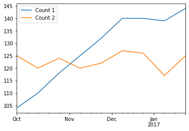
df = pd . DataFrame ({ 'Count 1' : 100 + np . random . randint ( - 5 , 10 , 9 ). cumsum (),
'Count 2' : 120 + np . random . randint ( - 5 , 10 , 9 )}, index = dates )
df
Count 1
Count 2
2016-10-02
104
125
2016-10-16
110
120
2016-10-30
118
124
2016-11-13
125
120
2016-11-27
132
122
2016-12-11
140
127
2016-12-25
140
126
2017-01-08
139
117
2017-01-22
144
125
Count 1
Count 2
2016-10-02
NaN
NaN
2016-10-16
6.0
-5.0
2016-10-30
8.0
4.0
2016-11-13
7.0
-4.0
2016-11-27
7.0
2.0
2016-12-11
8.0
5.0
2016-12-25
0.0
-1.0
2017-01-08
-1.0
-9.0
2017-01-22
5.0
8.0
Count 1
Count 2
2016-10-31
110.666667
123.0
2016-11-30
128.500000
121.0
2016-12-31
140.000000
126.5
2017-01-31
141.500000
121.0
C:\Users\LENOVO\AppData\Local\Temp/ipykernel_4900/1797912031.py:1: FutureWarning: Indexing a DataFrame with a datetimelike index using a single string to slice the rows, like `frame[string]`, is deprecated and will be removed in a future version. Use `frame.loc[string]` instead.
  df['2017']
Count 1
Count 2
2017-01-08
139
117
2017-01-22
144
125
C:\Users\LENOVO\AppData\Local\Temp/ipykernel_4900/2391205231.py:1: FutureWarning: Indexing a DataFrame with a datetimelike index using a single string to slice the rows, like `frame[string]`, is deprecated and will be removed in a future version. Use `frame.loc[string]` instead.
  df['2016-12']
Count 1
Count 2
2016-12-11
140
127
2016-12-25
140
126
Count 1
Count 2
2016-12-11
140
127
2016-12-25
140
126
2017-01-08
139
117
2017-01-22
144
125
df . asfreq ( 'W' , method = 'ffill' )
Count 1
Count 2
2016-10-02
104
125
2016-10-09
104
125
2016-10-16
110
120
2016-10-23
110
120
2016-10-30
118
124
2016-11-06
118
124
2016-11-13
125
120
2016-11-20
125
120
2016-11-27
132
122
2016-12-04
132
122
2016-12-11
140
127
2016-12-18
140
127
2016-12-25
140
126
2017-01-01
140
126
2017-01-08
139
117
2017-01-15
139
117
2017-01-22
144
125
import matplotlib.pyplot as plt
% matplotlib inline
df . plot ()
np . random . binomial ( 1 , 0.5 )
np . random . binomial ( 1000 , 0.5 ) / 1000
chance_of_tornado = 0.01 / 100
np . random . binomial ( 100000 , chance_of_tornado )
distribution = np . random . normal ( 0.75 , size = 1000 )
np . std ( distribution )
import scipy.stats as stats
stats . kurtosis ( distribution )
chi_squared_df2 = np . random . chisquare ( 2 , size = 10000 )
stats . skew ( chi_squared_df2 )
Applied data science with python by Michigan university, Coursera
Python for data analysis book by O’Reilly
Pandas Bootcamp by Udemy