Loading Real Image Data
For this section we’ll be working with a version of the Cats vs. Dogs dataset inspired by a classic Kaggle competition.
The images are similar to ones available from the ImageNet database.
We have organized the files into train and test folders, and further divided the images into CAT and DOG subfolders. In this way the file path contains the label.
Image files directory tree
.
└── Data
    └── CATS_DOGS
        ├── test
        │   ├── CAT
        │   │   ├── 9374.jpg
        │   │   ├── 9375.jpg
        │   │   └── ... (3,126 files)
        │   └── DOG
        │       ├── 9374.jpg
        │       ├── 9375.jpg
        │       └── ... (3,125 files)
        │
        └── train
            ├── CAT
            │   ├── 0.jpg
            │   ├── 1.jpg
            │   └── ... (9,371 files)
            └── DOG
                ├── 0.jpg
                ├── 1.jpg
                └── ... (9,372 files)
import glob
paths = glob.glob('../content/Data/CATS_DOGS/train/*.jpg')
paths[:5]
cat_images = list(filter(lambda x : x.split('/')[-1].split('.')[0] == 'cat', paths))
dog_images = list(filter(lambda x : x.split('/')[-1].split('.')[0] == 'dog', paths))
# split cat,dog data to train,test
train_size_cat = int(len(cat_images)*0.7)
print(train_size_cat)
train_size_dog = int(len(dog_images)*0.7)
print(train_size_dog)
8750
8750
Perform standard imports
import torch
import torch.nn as nn
import torch.nn.functional as F
from torch.utils.data import DataLoader
from torchvision import datasets, transforms

import numpy as np
import pandas as pd
import matplotlib.pyplot as plt
%matplotlib inline
Image Preprocessing
Any network we define requires consistent input data. That is, the incoming image files need to have the same number of channels (3 for red/green/blue), the same depth per channel (0-255), and the same height and width. This last requirement can be tricky. How do we transform an 800x450 pixel image into one that is 224x224? In the theory lectures we covered the following:
- aspect ratio: the ratio of width to height (16:9, 1:1, etc.) An 800x450 pixel image has an aspect ration of 16:9. We can change the aspect ratio of an image by cropping it, by stretching/squeezing it, or by some combination of the two. In both cases we lose some information contained in the original. Let’s say we crop 175 pixels from the left and right sides of our 800x450 image, resulting in one that’s 450x450.
- scale: Once we’ve attained the proper aspect ratio we may need to scale an image up or down to fit our input parameters. There are several libraries we can use to scale a 450x450 image down to 224x224 with minimal loss.
- normalization: when images are converted to tensors, the [0,255] rgb channels are loaded into range [0,1]. We can then normalize them using the generally accepted values of mean=[0.485, 0.456, 0.406] and std=[0.229, 0.224, 0.225]. For the curious, these values were obtained by the PyTorch team using a random 10,000 sample of ImageNet images. There’s a good discussion of this here, and the original source code can be found here.
Transformations
import os
from PIL import Image
from IPython.display import display

# Filter harmless warnings
import warnings
warnings.filterwarnings("ignore")
dog = Image.open('../content/Data/CATS_DOGS/train/DOG/1164.jpg')
print(dog.size)
display(dog)
(490, 499)

This is how jupyter displays the original .jpg image. Note that size is given as (width, height).
Let’s look at a single pixel:
r, g, b = dog.getpixel((0, 0))
print(r,g,b)
140 153 71
The pixel at position [0,0] (upper left) of the source image has an rgb value of (90,95,98). This corresponds to this color
Great! Now let’s look at some specific transformations.
transforms.ToTensor()
Converts a PIL Image or numpy.ndarray (HxWxC) in the range [0, 255] to a torch.FloatTensor of shape (CxHxW) in the range [0.0, 1.0]
transform = transforms.Compose([
    transforms.ToTensor()
])
im = transform(dog)
print(im.shape)
plt.imshow(np.transpose(im.numpy(), (1, 2, 0)));
torch.Size([3, 499, 490])

This is the same image converted to a tensor and displayed using matplotlib. Note that the torch dimensions follow [channel, height, width]
PyTorch automatically loads the [0,255] pixel channels to [0,1]:
\(\frac{140}{255}=0.5490\quad\frac{153}{255}=0.6000\quad\frac{71}{255}=0.2784\)
im[:,0,0]
tensor([0.5490, 0.6000, 0.2784])
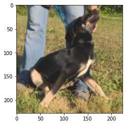
transforms.Resize(size)
If size is a sequence like (h, w), the output size will be matched to this. If size is an integer, the smaller edge of the image will be matched to this number.
i.e, if height > width, then the image will be rescaled to (size * height / width, size)
transform = transforms.Compose([
    transforms.Resize(224),
    transforms.ToTensor()
])
im = transform(dog)
print(im.shape)
plt.imshow(np.transpose(im.numpy(), (1, 2, 0)));
torch.Size([3, 228, 224])
transforms.CenterCrop(size)
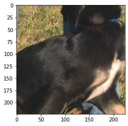
If size is an integer instead of sequence like (h, w), a square crop of (size, size) is made.
transform = transforms.Compose([
    transforms.CenterCrop(224),
    transforms.ToTensor()
])
im = transform(dog) # this crops the original image
print(im.shape)
plt.imshow(np.transpose(im.numpy(), (1, 2, 0)));
torch.Size([3, 224, 224])
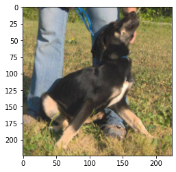
It may be better to resize the image first, then crop:
transform = transforms.Compose([
    transforms.Resize(224),
    transforms.CenterCrop(224),
    transforms.ToTensor()
])
im = transform(dog)
print(im.shape)
plt.imshow(np.transpose(im.numpy(), (1, 2, 0)));
torch.Size([3, 224, 224])
Other affine transformations
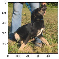
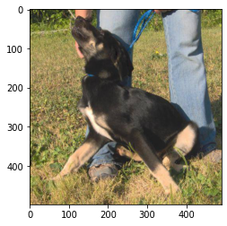
An affine transformation is one that preserves points and straight lines. Examples include rotation, reflection, and scaling. For instance, we can double the effective size of our training set simply by flipping the images.
transforms.RandomHorizontalFlip(p=0.5)
Horizontally flip the given PIL image randomly with a given probability.
transform = transforms.Compose([
    transforms.ToTensor()
])
im = transform(dog)
print(im.shape)
plt.imshow(np.transpose(im.numpy(), (1, 2, 0)));
torch.Size([3, 499, 490])
transform = transforms.Compose([
    transforms.RandomHorizontalFlip(p=1),  # normally we'd set p=0.5
    transforms.ToTensor()
])
im = transform(dog)
print(im.shape)
plt.imshow(np.transpose(im.numpy(), (1, 2, 0)));
torch.Size([3, 499, 490])
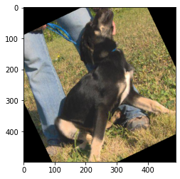
transforms.RandomRotation(degrees)
If degrees is a number instead of sequence like (min, max), the range of degrees will be (-degrees, +degrees).
Run the cell below several times to see a sample of rotations.
transform = transforms.Compose([
    transforms.RandomRotation(30),  # rotate randomly between +/- 30 degrees
    transforms.ToTensor()
])
im = transform(dog)
print(im.shape)
plt.imshow(np.transpose(im.numpy(), (1, 2, 0)));
torch.Size([3, 499, 490])
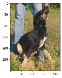
Scaling is done using transforms.Resize(size)
transform = transforms.Compose([
    transforms.Resize((300,224)),  # be sure to pass in a list or a tuple
    transforms.ToTensor()
])
im = transform(dog)
print(im.shape)
plt.imshow(np.transpose(im.numpy(), (1, 2, 0)));
torch.Size([3, 300, 224])
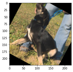
Let’s put it all together
transform = transforms.Compose([
    transforms.RandomHorizontalFlip(p=1),  # normally we'd set p=0.5
    transforms.RandomRotation(30),
    transforms.Resize(224),
    transforms.CenterCrop(224),
    transforms.ToTensor()
])
im = transform(dog)
print(im.shape)
plt.imshow(np.transpose(im.numpy(), (1, 2, 0)));
torch.Size([3, 224, 224])
Normalization
Once the image has been loaded into a tensor, we can perform normalization on it. This serves to make convergence happen quicker during training. The values are somewhat arbitrary - you can use a mean of 0.5 and a standard deviation of 0.5 to convert a range of [0,1] to [-1,1], for example.
However, research has shown that mean=[0.485, 0.456, 0.406] and std=[0.229, 0.224, 0.225] work well in practice.
transforms.Normalize(mean, std)
Given mean: (M1,…,Mn) and std: (S1,..,Sn) for n channels, this transform will normalize each channel of the input tensor
\(\quad\textrm {input[channel]} = \frac{\textrm{input[channel] - mean[channel]}}{\textrm {std[channel]}}\)
transform = transforms.Compose([
    transforms.ToTensor(),
    transforms.Normalize([0.485, 0.456, 0.406],
                         [0.229, 0.224, 0.225])
])
im = transform(dog)
print(im.shape)
plt.imshow(np.transpose(im.numpy(), (1, 2, 0)));
Clipping input data to the valid range for imshow with RGB data ([0..1] for floats or [0..255] for integers).


torch.Size([3, 499, 490])

Recall that before normalization, the upper-leftmost tensor had pixel values of [0.5490, 0.6000, 0.2784].
With normalization we subtract the channel mean from the input channel, then divide by the channel std.
\(\frac{(0.5490-0.485)}{0.229}=0.2857\quad\frac{(0.6000-0.456)}{0.224}=0.6429\quad\frac{(0.2784-0.406)}{0.225}=-0.5670\)
# After normalization:
im[:,0,0]
tensor([ 0.2796, 0.6429, -0.5670])
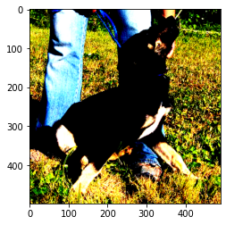
When displayed, matplotlib clipped this particular pixel up to [0,0,0] so it appears black on the screen. However, the appearance isn’t important; the goal of normalization is improved mathematical performance.
Optional: De-normalize the images
To see the image back in its true colors, we can apply an inverse-transform to the tensor being displayed.
inv_normalize = transforms.Normalize(
    mean=[-0.485/0.229, -0.456/0.224, -0.406/0.225],
    std=[1/0.229, 1/0.224, 1/0.225]
)
im_inv = inv_normalize(im)
plt.figure(figsize=(12,4))
plt.imshow(np.transpose(im_inv.numpy(), (1, 2, 0)));

Note that the original tensor was not modified:
plt.figure(figsize=(12,4))
plt.imshow(np.transpose(im.numpy(), (1, 2, 0)));
Clipping input data to the valid range for imshow with RGB data ([0..1] for floats or [0..255] for integers).
More detailed documentation on transforming and augmenting images using PyTorch is described in here.